Introduction
This document may be temporarily meaningful because the functionality will be included in NonCompart (Bae 2017) package someday as Prof.Bae said. Until then, I hope that these tips can save several minutes (or hours) for a few people.
One thing we should keep in mind is that the output of tblNCA() is a character matrix so we probably want to change it to data.frame (or tibble) for the further manipulation and the PK parameters should be converted to numeric by as.numeric() to find descriptive statistics.
These R packages are used.
library(NonCompart) # for tblNCA(), IntAUC()
library(dplyr) # for data manipulation
library(tidyr) # for data manipulation
library(purrr) # for pmap_dbl()
library(knitr) # make pretty tables (can be ignored when we don't need them.)
How to include iAUC in the tblNCA
Writing tblNCA2()
tblNCA2() is a wrapper function of tblNCA() to include iAUC. In the function, iAUC is calculated by IntAUC(). Data manipulation can be done in numerous ways but I prefer using Hadley’s packages for functional programming (Henry and Wickham 2017) and tidy data handling (Wickham and Henry 2017; Wickham et al. 2017).
tblNCA2 <- function(concData, key = "Subject",
                    colTime = "Time", colConc = "conc",
                    down = "linear", t1 = 0, t2 = 0, ...){
  # tblNCA() and data calculation
  input_tbl <- tblNCA(as.data.frame(concData),
                      key, colTime, colConc, down = down, ...) %>% # calculation
    as_tibble() %>% mutate_all(as.character) %>%
    left_join(concData %>%
                as_tibble() %>% mutate_all(as.character) %>%
                group_by_(.dots = key) %>% # grouping by keys (Subject)
                summarise_(x = sprintf('list(%s)', colTime),
                           y = sprintf('list(%s)', colConc)))

  # calculation of IntAUC()
  output <- input_tbl %>%
    mutate(Res = do.call(c, input_tbl %>% select(-x, -y) %>% apply(1, list))) %>%
    mutate(iAUC = pmap_dbl(.l = list(x, y, Res),
                           .f = ~IntAUC(x = as.numeric(..1), y = as.numeric(..2),
                                        t1, t2,
                                        Res = ..3, down = down))) %>%
    select(-x, -y, -Res) %>%
    mutate_at(vars(b0:iAUC), as.numeric) # character -> number
  return(output)
}
Examples
Example 1: datasets::Theoph
Now we can use tblNCA2() to find NCA parameters and interval AUC between 0-12 hours of Theoph dataset internally available in R.
Theoph_with_iAUC <- tblNCA2(Theoph, dose = 320, t1 = 0, t2 = 12) # 0-12h
Theoph_with_iAUC %>%
kable(caption = 'Entire PK parameters calculated by NonCompart', booktabs=TRUE, digits = 2)| Subject | b0 | CMAX | CMAXD | TMAX | TLAG | CLST | CLSTP | TLST | LAMZHL | LAMZ | LAMZLL | LAMZUL | LAMZNPT | CORRXY | R2 | R2ADJ | AUCLST | AUCALL | AUCIFO | AUCIFOD | AUCIFP | AUCIFPD | AUCPEO | AUCPEP | AUMCLST | AUMCIFO | AUMCIFP | AUMCPEO | AUMCPEP | VZFO | VZFP | CLFO | CLFP | MRTEVLST | MRTEVIFO | MRTEVIFP | iAUC |
|---|---|---|---|---|---|---|---|---|---|---|---|---|---|---|---|---|---|---|---|---|---|---|---|---|---|---|---|---|---|---|---|---|---|---|---|---|---|
| 1 | 2.37 | 10.50 | 0.03 | 1.12 | 0 | 3.28 | 3.28 | 24.37 | 14.30 | 0.05 | 9.05 | 24.37 | 3 | -1 | 1.00 | 1.00 | 148.92 | 148.92 | 216.61 | 0.68 | 216.61 | 0.68 | 31.25 | 31.25 | 1459.07 | 4505.53 | 4505.67 | 67.62 | 67.62 | 30486.75 | 30486.32 | 1477.30 | 1477.28 | 9.80 | 20.80 | 20.80 | 91.74 |
| 2 | 2.41 | 8.33 | 0.03 | 1.92 | 0 | 0.90 | 0.89 | 24.30 | 6.66 | 0.10 | 7.03 | 24.30 | 4 | -1 | 1.00 | 1.00 | 91.53 | 91.53 | 100.17 | 0.31 | 100.06 | 0.31 | 8.63 | 8.53 | 706.59 | 999.77 | 996.07 | 29.33 | 29.06 | 30690.44 | 30723.92 | 3194.46 | 3197.94 | 7.72 | 9.98 | 9.95 | 67.48 |
| 3 | 2.53 | 8.20 | 0.03 | 1.02 | 0 | 1.05 | 1.06 | 24.17 | 6.77 | 0.10 | 9.00 | 24.17 | 3 | -1 | 1.00 | 1.00 | 99.29 | 99.29 | 109.54 | 0.34 | 109.59 | 0.34 | 9.36 | 9.40 | 803.19 | 1150.96 | 1152.65 | 30.22 | 30.32 | 28517.10 | 28504.15 | 2921.41 | 2920.09 | 8.09 | 10.51 | 10.52 | 70.18 |
| 4 | 2.59 | 8.60 | 0.03 | 1.07 | 0 | 1.15 | 1.16 | 24.65 | 6.98 | 0.10 | 9.02 | 24.65 | 3 | -1 | 1.00 | 1.00 | 106.80 | 106.80 | 118.38 | 0.37 | 118.44 | 0.37 | 9.78 | 9.83 | 901.08 | 1303.25 | 1305.50 | 30.86 | 30.98 | 27225.96 | 27211.10 | 2703.18 | 2701.71 | 8.44 | 11.01 | 11.02 | 73.05 |
| 5 | 2.55 | 11.40 | 0.04 | 1.00 | 0 | 1.57 | 1.56 | 24.35 | 8.00 | 0.09 | 7.02 | 24.35 | 4 | -1 | 1.00 | 1.00 | 121.29 | 121.29 | 139.42 | 0.44 | 139.25 | 0.44 | 13.00 | 12.90 | 1017.11 | 1667.72 | 1661.79 | 39.01 | 38.79 | 26497.99 | 26529.42 | 2295.23 | 2297.95 | 8.39 | 11.96 | 11.93 | 84.61 |
| 6 | 2.03 | 6.44 | 0.02 | 1.15 | 0 | 0.92 | 0.94 | 23.85 | 7.89 | 0.09 | 2.03 | 23.85 | 7 | -1 | 1.00 | 1.00 | 73.78 | 73.78 | 84.25 | 0.26 | 84.50 | 0.26 | 12.44 | 12.69 | 609.15 | 978.43 | 986.97 | 37.74 | 38.28 | 43259.73 | 43135.69 | 3798.02 | 3787.13 | 8.26 | 11.61 | 11.68 | 51.76 |
| 7 | 2.29 | 7.09 | 0.02 | 3.48 | 0 | 1.15 | 1.16 | 24.22 | 7.85 | 0.09 | 6.98 | 24.22 | 4 | -1 | 1.00 | 1.00 | 90.75 | 90.75 | 103.77 | 0.32 | 103.89 | 0.32 | 12.55 | 12.65 | 782.42 | 1245.10 | 1249.41 | 37.16 | 37.38 | 34908.44 | 34867.67 | 3083.69 | 3080.09 | 8.62 | 12.00 | 12.03 | 62.10 |
| 8 | 2.17 | 7.56 | 0.02 | 2.02 | 0 | 1.25 | 1.23 | 24.12 | 8.51 | 0.08 | 3.53 | 24.12 | 6 | -1 | 0.99 | 0.99 | 88.56 | 88.56 | 103.91 | 0.32 | 103.64 | 0.32 | 14.77 | 14.55 | 739.53 | 1298.12 | 1288.52 | 43.03 | 42.61 | 37810.51 | 37906.69 | 3079.69 | 3087.52 | 8.35 | 12.49 | 12.43 | 62.71 |
| 9 | 2.12 | 9.03 | 0.03 | 0.63 | 0 | 1.12 | 1.12 | 24.43 | 8.41 | 0.08 | 8.80 | 24.43 | 3 | -1 | 1.00 | 1.00 | 86.33 | 86.33 | 99.91 | 0.31 | 99.87 | 0.31 | 13.59 | 13.56 | 705.23 | 1201.77 | 1200.21 | 41.32 | 41.24 | 38842.79 | 38859.38 | 3202.92 | 3204.29 | 8.17 | 12.03 | 12.02 | 60.12 |
| 10 | 2.66 | 10.21 | 0.03 | 3.55 | 0 | 2.42 | 2.41 | 23.70 | 9.25 | 0.07 | 9.38 | 23.70 | 3 | -1 | 1.00 | 1.00 | 138.37 | 138.37 | 170.65 | 0.53 | 170.57 | 0.53 | 18.92 | 18.88 | 1278.18 | 2473.99 | 2470.88 | 48.34 | 48.27 | 25015.54 | 25027.88 | 1875.16 | 1876.09 | 9.24 | 14.50 | 14.49 | 90.82 |
| 11 | 2.15 | 8.00 | 0.02 | 0.98 | 0 | 0.86 | 0.86 | 24.08 | 7.26 | 0.10 | 9.03 | 24.08 | 3 | -1 | 1.00 | 1.00 | 80.09 | 80.09 | 89.10 | 0.28 | 89.10 | 0.28 | 10.11 | 10.11 | 617.24 | 928.56 | 928.49 | 33.53 | 33.52 | 37622.19 | 37623.04 | 3591.36 | 3591.44 | 7.71 | 10.42 | 10.42 | 58.54 |
| 12 | 2.82 | 9.75 | 0.03 | 3.52 | 0 | 1.17 | 1.18 | 24.15 | 6.29 | 0.11 | 9.03 | 24.15 | 3 | -1 | 1.00 | 1.00 | 119.98 | 119.98 | 130.59 | 0.41 | 130.64 | 0.41 | 8.13 | 8.16 | 977.88 | 1330.38 | 1332.05 | 26.50 | 26.59 | 22224.29 | 22215.75 | 2450.44 | 2449.50 | 8.15 | 10.19 | 10.20 | 85.02 |
Table 1 is so wide that we may want to focus on Cmax, Tmax, AUClast, AUCinf, and iAUC. Table 2 looks okay. We can compare the values with the concentration-time curves in Figure 1
Theoph_with_iAUC_selected <- Theoph_with_iAUC %>%
  select(Subject, CMAX, TMAX, AUCLST, AUCIFO, iAUC)

Theoph_with_iAUC_selected %>%
kable(caption = 'Selected PK parameters including iAUC', booktabs=TRUE, digits = 2)| Subject | CMAX | TMAX | AUCLST | AUCIFO | iAUC |
|---|---|---|---|---|---|
| 1 | 10.50 | 1.12 | 148.92 | 216.61 | 91.74 |
| 2 | 8.33 | 1.92 | 91.53 | 100.17 | 67.48 |
| 3 | 8.20 | 1.02 | 99.29 | 109.54 | 70.18 |
| 4 | 8.60 | 1.07 | 106.80 | 118.38 | 73.05 |
| 5 | 11.40 | 1.00 | 121.29 | 139.42 | 84.61 |
| 6 | 6.44 | 1.15 | 73.78 | 84.25 | 51.76 |
| 7 | 7.09 | 3.48 | 90.75 | 103.77 | 62.10 |
| 8 | 7.56 | 2.02 | 88.56 | 103.91 | 62.71 |
| 9 | 9.03 | 0.63 | 86.33 | 99.91 | 60.12 |
| 10 | 10.21 | 3.55 | 138.37 | 170.65 | 90.82 |
| 11 | 8.00 | 0.98 | 80.09 | 89.10 | 58.54 |
| 12 | 9.75 | 3.52 | 119.98 | 130.59 | 85.02 |
library(ggplot2)
ggplot(Theoph %>% left_join(Theoph_with_iAUC), aes(x = Time, y = conc)) +
  geom_line() +
  geom_point(color = 'red') +
  facet_wrap(~ sprintf('Subject %2s,Cmax %0.1f,\nAUClast %0.1f,iAUC %0.1f',
                       Subject, CMAX, AUCLST, iAUC), ncol = 4) +
  scale_x_continuous(breaks = c(0, 6, 12, 24)) +
  theme_minimal()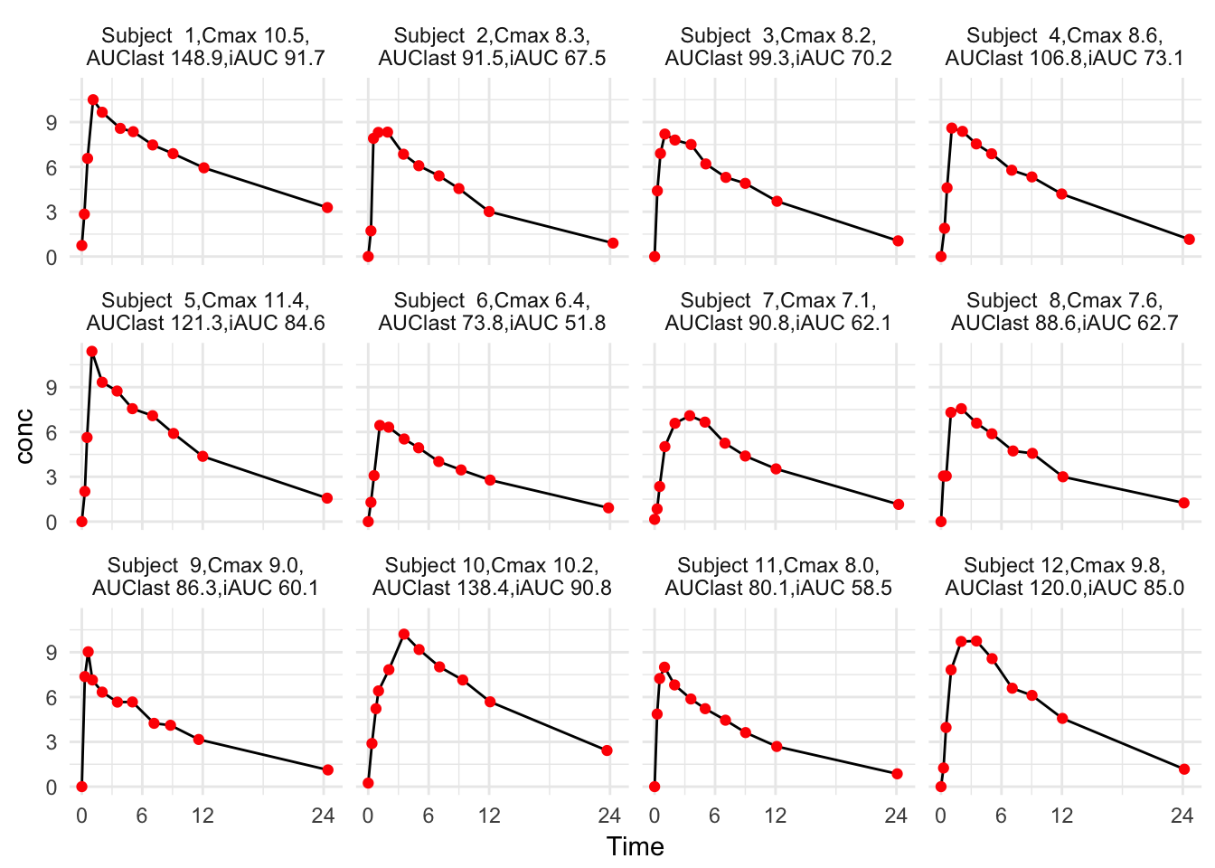
Figure 1: Individual concentration-time curves
Example 2: PKPDdatasets::sd_oral_richpk
PKPDdatasets package (Pastoor 2014) contains some interesting PK/PD datasets and I want to apply tblNCA2() to one of them. In this case, I’ll add some more keys such as gender and race. Factors should be converted to characters and strangely the lower case should be avoided as a input of keys in tblNCA(). Table 3 shows the results and multiple keys are working fine. Results of only 10 subjects are shown here out of total 50 subjects.
sd_oral_richpk_char <- PKPDdatasets::sd_oral_richpk %>%
  filter(ID <= 12) %>%
  mutate_at(vars(ID, Gender, Race), function(x) toupper(as.character(x)))

tblNCA2(sd_oral_richpk_char,
        key = c('ID', 'Gender', 'Race'), 'Time', 'Conc', dose = 5000, t1 = 0, t2 = 12) %>%
  select(ID, Gender, Race, CMAX, TMAX, AUCLST, AUCIFO, iAUC) %>%
  kable(caption = 'Selected PK parameters including iAUC of sd oral richpk',
booktabs=TRUE, digits = 2)| ID | Gender | Race | CMAX | TMAX | AUCLST | AUCIFO | iAUC |
|---|---|---|---|---|---|---|---|
| 1 | MALE | HISPANIC | 34.01 | 1 | 385.58 | 449.44 | 280.59 |
| 2 | MALE | CAUCASIAN | 100.18 | 2 | 1203.49 | 2495.10 | 732.30 |
| 3 | MALE | OTHER | 53.86 | 3 | 466.31 | 481.99 | 389.24 |
| 4 | FEMALE | CAUCASIAN | 96.68 | 4 | 1219.64 | 1789.21 | 775.31 |
| 5 | FEMALE | CAUCASIAN | 51.63 | 2 | 487.57 | 516.44 | 385.18 |
| 6 | MALE | HISPANIC | 27.94 | 4 | 295.25 | 342.57 | 208.93 |
| 7 | MALE | OTHER | 71.81 | 4 | 739.03 | 876.99 | 521.99 |
| 8 | MALE | ASIAN | 44.45 | 3 | 453.77 | 472.76 | 345.15 |
| 9 | FEMALE | OTHER | 48.47 | 4 | 698.99 | 817.67 | 435.38 |
| 10 | MALE | OTHER | 23.52 | 2 | 161.45 | 162.89 | 146.59 |
| 11 | MALE | ASIAN | 68.10 | 6 | 962.56 | 1272.65 | 611.06 |
| 12 | MALE | OTHER | 83.63 | 2 | 721.85 | 768.82 | 550.52 |
How to get descriptive statistics
You may want to use psych::describe() or broom::tidy() (Robinson 2017). They returns basically the same results. One thing to be mentioned is that broom::tidy() returns the descriptive statistics when the input is data.frame so as.data.frame() should be first applied to the output of tblNCA(). (Table 4)
broom::tidy(as.data.frame(Theoph_with_iAUC_selected)) %>%
  kable(caption = 'Descriptive statistics of selected PK parameters of Theoph',
booktabs = TRUE, digits = 2)| column | n | mean | sd | median | trimmed | mad | min | max | range | skew | kurtosis | se |
|---|---|---|---|---|---|---|---|---|---|---|---|---|
| Subject* | 12 | 6.50 | 3.61 | 6.50 | 6.50 | 4.45 | 1.00 | 12.00 | 11.00 | 0.00 | -1.50 | 1.04 |
| CMAX | 12 | 8.76 | 1.47 | 8.46 | 8.73 | 1.62 | 6.44 | 11.40 | 4.96 | 0.21 | -1.19 | 0.43 |
| TMAX | 12 | 1.79 | 1.11 | 1.14 | 1.73 | 0.49 | 0.63 | 3.55 | 2.92 | 0.70 | -1.35 | 0.32 |
| AUCLST | 12 | 103.81 | 23.65 | 95.41 | 102.30 | 19.79 | 73.78 | 148.92 | 75.15 | 0.56 | -1.12 | 6.83 |
| AUCIFO | 12 | 122.19 | 38.13 | 106.72 | 116.54 | 21.70 | 84.25 | 216.61 | 132.36 | 1.25 | 0.51 | 11.01 |
| iAUC | 12 | 71.51 | 13.52 | 68.83 | 71.46 | 14.08 | 51.76 | 91.74 | 39.98 | 0.24 | -1.55 | 3.90 |
Write your own scripts
You can write some codes to customize the descriptive statistics.
Theoph_tblNCA <- tblNCA(Theoph)

as_tibble(Theoph_tblNCA) %>%
  gather(PPTESTCD, PPORRES, -Subject) %>%
  left_join(tibble(PPTESTCD = attr(Theoph_tblNCA, 'dimnames')[[2]],
                   UNIT = attr(Theoph_tblNCA, 'units')),
          by = 'PPTESTCD') %>%
  mutate(PPORRES = as.numeric(PPORRES)) %>%
  group_by(PPTESTCD, UNIT) %>%
  summarise_at(vars(PPORRES), funs(n(), mean, sd, cv = sd/mean*100,
                                   geomean = PKNCA::geomean,
                                   geosd = PKNCA::geosd,
                                   geocv = PKNCA::geocv,
                                   median, min, max)) %>%
  mutate(`Arithmetic mean ± SD (CV%)` = sprintf('%0.1f ± %0.1f (%0.1f%%)', mean, sd, cv)) %>%
  mutate(`Geometric mean ± SD (CV%)` = sprintf('%0.1f ± %0.1f (%0.1f%%)', geomean, geosd, geocv)) %>%
  mutate(`Median [range]` = sprintf('%0.1f [%0.1f-%0.1f]', median, min, max)) %>%
  select(-mean, -sd, -cv, -geomean, -geosd, -geocv, -median, -min, -max) %>%
  filter(PPTESTCD %in% c('CMAX', 'TMAX', 'AUCLST', 'AUCIFO')) %>%
  kable(caption = 'Descriptive statistics of selected PK parameters manually calculated.',
booktabs = TRUE) | PPTESTCD | UNIT | n | Arithmetic mean ± SD (CV%) | Geometric mean ± SD (CV%) | Median [range] |
|---|---|---|---|---|---|
| AUCIFO | h*ug/L | 12 | 122.2 ± 38.1 (31.2%) | 117.7 ± 1.3 (28.0%) | 106.7 [84.3-216.6] |
| AUCLST | h*ug/L | 12 | 103.8 ± 23.6 (22.8%) | 101.5 ± 1.2 (22.3%) | 95.4 [73.8-148.9] |
| CMAX | ug/L | 12 | 8.8 ± 1.5 (16.8%) | 8.6 ± 1.2 (17.0%) | 8.5 [6.4-11.4] |
| TMAX | h | 12 | 1.8 ± 1.1 (62.2%) | 1.5 ± 1.8 (64.7%) | 1.1 [0.6-3.5] |
Although there’s an advantage of customization, the script is quite lengthy, so unless you’re preparing a journal paper, I just recommend using broom::tidy().
References
Bae, Kyun-Seop. 2017. NonCompart: Noncompartmental Analysis for Pharmacokinetic Data. https://CRAN.R-project.org/package=NonCompart.
Henry, Lionel, and Hadley Wickham. 2017. Purrr: Functional Programming Tools. https://CRAN.R-project.org/package=purrr.
Pastoor, Devin. 2014. PKPDdatasets: Data Sets for Pharmacometric Analysis and Visualization.
Robinson, David. 2017. Broom: Convert Statistical Analysis Objects into Tidy Data Frames. https://CRAN.R-project.org/package=broom.
Wickham, Hadley, and Lionel Henry. 2017. Tidyr: Easily Tidy Data with ’Spread()’ and ’Gather()’ Functions. https://CRAN.R-project.org/package=tidyr.
Wickham, Hadley, Romain Francois, Lionel Henry, and Kirill Müller. 2017. Dplyr: A Grammar of Data Manipulation. https://CRAN.R-project.org/package=dplyr.